Motion & Tracking

1. Recall: Histograms of oriented gradients (HOG)

Partition image into blocks and compute histogram of gradient orientations in each block

对光照不敏感，一定程度上可以容忍一些变化

1.1 Pedestrian detection with HOG

Train a pedestrian template using a linear support vector machine

At test time, convolve feature map with template(SVM)
Find local maxima of response
For multi-scale detection, repeat over multiple levels of a HOG pyramid

1.2 Window-based detection: strengths

Sliding window detection and global appearance descriptors: Simple detection
- protocol to implement
- Good feature choices critical
- Past successes for certain classes

1.3 High computational complexity

For example: 250,000 locations x 30 orientations x 4 scales = 30,000,000 evaluations!
If training binary detectors independently, means cost increases linearly with number of classes
对于一些方形的框不能有针对进行目标检测，因为物体不一定都是呈矩形分布的
Non-rigid, deformable（非刚性的、可变形的物体） objects not captured well with representations assuming a fixed 2d structure; or must assume fixed viewpoint
- 对非刚性形变不具有鲁棒性

If considering windows in isolation, context is lost、
- 丢失上下文信息

In practice, often entails large, cropped training set (expensive)
Requiring good match to a global appearance description can lead to sensitivity to partial occlusions
- 需要标记

2. Discriminative part-based models

Single rigid template usually not enough to represent a category
- Many objects (e.g. humans) are articulated(铰接式), or have parts that can vary in configuration(结构)

Many object categories look very different from different viewpoints, or from instance to instance
- 不同视角带来的变化

2.1 Solution

先用全局做响应，再用局部算子做相应
不管是哪个部分存在，都可以判定为目标检测成功

虽然空间组合发生变化，但是部件仍能检测出来

3. Object proposals

3.1 Main idea:

Learn to generate category-independent regions/boxes that have object-like properties.
Let object detector search over “proposals”, not exhaustive sliding windows
- 找有目标的窗口

多尺度显著性
- 人眼在观测物体时，会有关注点

颜色对比度
- 一般物体检测周围环境的颜色存在明显的变化

边缘密度，一般来说一个物体的边缘是闭合的

超像素跨越性：把相似的像素点聚类在一起叫超像素，一个超像素不应该属于两个类。一个框不可能跨越超像素，否则框内无目标

只需要1000个窗口，就能把目标框出来

3.2 Summary

Object recognition as classification task
- Boosting (face detection ex)
- Support vector machines and HOG (person detection ex)
- Sliding window search paradigm
  - Pros and cons
  - Speed up with attentional cascade
  - Discriminative part-based models, object proposals

4. Motion and Tracking

4.1 From images to videos

A video is a sequence of frames captured over time
Now our image data is a function of space (𝑥,𝑦)and time (𝑡)

4.2 Motion is a powerful perceptual cue

Sometimes, it is the only cue
- 每一帧图片具有强相关性，运动可以带来丰富的信息
- 下图在运动时可以看到两个圆

Even “impoverished” motion data can evoke a strong percept
- 下图可以看出一个运动的人

4.3 Uses of motion in computer vision

3D shape reconstruction
- 多角度拍摄
Object segmentation
Learning and tracking of dynamical models
- 目标追踪
Event and activity recognition

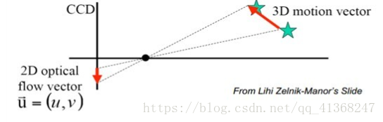
4.4 Motion field

motion field is the projection of the 3D scene motion into the image
- 运动场是3D场景运动到图像中的投影

4.5 Motion estimation: Optical flow

Definition: optical flow is the apparent motion of brightness patterns in the image
- 明显亮度模式的运动
- 光流（optical flow）是空间运动物体在观察成像平面上的像素运动的瞬时速度。
Ideally, optical flow would be the same as the motion field
Have to be careful: apparent motion can be caused by lighting changes without any actual motion
- Think of a uniform rotating sphere under fixed lighting vs. a stationary sphere under moving illumination
- 一种是均匀光照对选装球体的影响
- 一种是光照变化，但是物体不动
GOAL:Recover image motion at each pixel from optical flow

4.6 Estimating optical flow

时间很小，位移矢量近似于速度矢量
Given two subsequent frames, estimate the apparent motion field u(x,y), v(x,y) between them
- u,v分别是横向速度和纵向速度

Key assumptions
- Brightness constancy: projection of the same point looks the same in every frame
  - 亮度恒定不变。相同的投影点在不同帧间运动时，其亮度不会发生改变。
- Small motion:points do not move very far
  - 时间连续或运动是“小运动”。即时间的变化不会引起目标位置的剧烈变化，相邻帧之间位移要比较小。
- Spatial coherence:points move like their neighbors
  - 空间相关性：相邻的点相似

4.6.1 Key Assumptions: small motions

相邻帧，某个区域的像素是逐渐变化的

4.6.2 Key Assumptions: spatial coherence

空间上的一致性，在小领域上运动趋势是相似的

4.6.3 Key Assumptions: brightness Constancy

4.7 The brightness constancy constraint

亮度恒定

$I(x, y, t-1)=I(x+u(x, y), y+v(x, y), t)$

Brightness Constancy Equation: $I(x, y, t-1)=I(x+u(x, y), y+v(x, y), t)$
Linearizing the right side using Taylor expansion:

$\begin{aligned} &\quad I(x+u, y+v, t) \approx I(x, y, t-1)+I_{x}u(x, y)+I_{y} v(x, y)+I_{t} \\ \\ &\quad I(x+u, y+v, t)-I(x, y, t-1)=I_{x} \cdot u(x, y)+I_{y} \cdot v(x, y)+I_{t} \\ \\ &\text { Hence, } \quad I_{x} \cdot u+I_{y} \cdot v+I_{t} \approx 0 \rightarrow \nabla I \cdot[u ,v]^{T}+I_{t}=0 \end{aligned}$

t方向求导即为：

$F_t=\left[\begin{array}{cc} 1 & 1\\ 1 & 1 \end{array}\right]，\ F_{t-1}=\left[\begin{array}{cc} -1 & -1\\ -1 & -1 \end{array}\right]$

Can we use this equation to recover image motion (u,v) at each pixel?

$\nabla I \cdot[u, v]^{T}+I_{t}=0$

增量和梯度方向垂直的话，增量就无影响

$\nabla I \cdot[u, v]^{T}=0,\text{for any u, v, if }\nabla I \perp [u,v]$

How many equations and unknowns per pixel?
- One equation (this is a scalar equation!), two unknowns (u,v)
- 无法求解参数
The component of the flow perpendicular（垂直） to the gradient (i.e., parallel to the edge) cannot be measured

会有多个解，与实际运动就会不一致

4.8 The aperture problem

孔径问题指在运动估计（Motion Estimation）中无法通过单个算子【计算某个像素值变化的操作，例如：梯度】准确无误地评估物体的运行轨迹。原因是每一个算子只能处理它所负责局部区域的像素值变化，然而同一种像素值变化可能是由物体的多种运行轨迹导致。

在小孔里看是平行运动，但实际三维运动却不是

三维是旋转，但是二维看起来是向上走
這就是「區域(local)」和「全域 (global)」視覺處理的差別。我們的視覺系統區域上 (locally) 可以有孔徑問題的錯覺，但是當我們觀察的範圍是全域 (globally)的時候，卻又分析的出來三張紙條不同的移動方向。

4.9 Solving the ambiguity

How to get more equations for a pixel?
Spatial coherence constraint:
- Assume the pixel’s neighbors have the same (u,v)
- If we use a 5x5 window, that gives us 25 equations per pixel

$\begin{gathered} 0=I_{t}\left(\mathrm{p}_{\mathrm{i}}\right)+\nabla I\left(\mathrm{p}_{\mathrm{i}}\right) \cdot\left[\begin{array}{ll} u & v \end{array}\right] \\ \\ {\left[\begin{array}{cc} I_{x}\left(\mathrm{p}_{1}\right) & I_{y}\left(\mathrm{p}_{1}\right) \\ I_{x}\left(\mathrm{p}_{2}\right) & I_{y}\left(\mathrm{p}_{2}\right) \\ \vdots & \vdots \\ I_{x}\left(\mathrm{p}_{25}\right) & I_{y}\left(\mathrm{p}_{25}\right) \end{array}\right]\left[\begin{array}{l} u \\ v \end{array}\right]=-\left[\begin{array}{c} I_{t}\left(\mathrm{p}_{1}\right) \\ I_{t}\left(\mathrm{p}_{2}\right) \\ \vdots \\ I_{t}\left(\mathrm{p}_{25}\right) \end{array}\right]} \end{gathered}$

Overconstrained linear system

$\left[\begin{array}{cc} I_{x}\left(\mathrm{p}_{1}\right) & I_{y}\left(\mathrm{p}_{1}\right) \\ I_{x}\left(\mathrm{p}_{2}\right) & I_{y}\left(\mathrm{p}_{2}\right) \\ \vdots & \vdots \\ I_{x}\left(\mathrm{p}_{25}\right) & I_{y}\left(\mathrm{p}_{25}\right) \end{array}\right]\left[\begin{array}{l} u \\ v \end{array}\right]=-\left[\begin{array}{c} I_{t}\left(\mathrm{p}_{1}\right) \\ I_{t}\left(\mathrm{p}_{2}\right) \\ \vdots \\ I_{t}\left(\mathrm{p}_{25}\right) \end{array}\right] \quad \begin{array}{cc} A & d=b \\ 25 \times 2 & 2 \times 1 \end{array}$

Least squares solution for $d$ given by $\left(A^{T} A\right) d=A^{T} b$

$\begin{gathered} {\left[\begin{array}{cc} \sum I_{x} I_{x} & \sum I_{x} I_{y} \\ \sum I_{x} I_{y} & \sum I_{y} I_{y} \end{array}\right]\left[\begin{array}{l} u \\ v \end{array}\right]=-\left[\begin{array}{c} \sum I_{x} I_{t} \\ \sum I_{y} I_{t} \end{array}\right]} \\ A^{T} A \end{gathered}$

The summations are over all pixels in the $\mathrm{K} \times \mathrm{K}$ window
Optimal $(u, v)$ satisfies Lucas-Kanade equation

When is this solvable? I.e., what are good points to track?
- $A^TA$ should be invertible
  - 不一定可逆
- $A^TA$ should not be too small due to noise
  - eigenvalues $\lambda_{1}$ and $\lambda_{2}$ of $A^{\top} A$ should not be too small
  - 如果$A^TA$值很小，如果有噪音，就会造成很大的扰动，所以特征值不能太小
- $A^TA$ should be well-conditioned
  - $\lambda_{1} / \lambda_{2}$ should not be too large $\left(\lambda_{1}=\right.$ larger eigenvalue $)$
Does this remind you of anything?
- Criteria for Harris corner detector

4.10 Recall: second moment matrix

Estimation of optical flow is well-conditioned precisely for regions with high “cornerness”:

4.10.1 Low texture region

对于平滑区域和边缘都不好检测光流估计
角点会较为容易检测，因为他的梯度在各个方向都有变化

4.10.2 The aperture problem resolved

用找交点的方式，来进行约束

4.11 Errors in Lucas-Kanade

The motion is large (larger than a pixel)
A point does not move like its neighbors
- 柔性物体的变化
Brightness constancy does not hold

Revisiting the small motion assumption

Is this motion small enough?
- Probably not—it’s much larger than one pixel
- How might we solve this problem?
意思是对于一些比较大的运动怎么进行测量？

4.12 Reduce the resolution!

利用下采样，那么原来偏移两个像素的运动，就会变成偏移一个像素，从而提高鲁棒性

4.13 Coarse-to-fine optical flow estimation

先将图片进行下采样

然后从最低分辨率的图片开始进行光流估计，然后在进行上采样
- 对于低分辨率求得的u,v将作为下一层的初始值

4.14 A point does not move like its neighbors

Motion segmentation

先分块，再用聚类的方法，找真正的方向，把图像分为不同的层，作为整体目标的考虑
Brightness constancy does not hold
- Feature matching
先检测关键点，就可以追踪关键点的轨迹

5. Feature Tracking

通过找到图像的关键点，然后最终图像关键点，从而形成特征追踪

5.1 Single object tracking

可以有效的解决遮挡问题

5.2 Multiple object tracking

可能遇到的问题
- 实体重叠
- 实体分开（id不能搞混）

5.3 Tracking with a fixed camera

因为用固定的相机拍摄，当人运动时会导致尺度会发生变化

5.4 Tracking with a moving camera

运动的相机背景发生变化

5.5 Tracking with multiple cameras

角度变化

5.6 Challenges in Feature tracking

Figure out which features can be tracked
- Efficiently track across frames
Some points may change appearance over time
- e.g., due to rotation, moving into shadows, etc.
Drift: small errors can accumulate as appearance model is updated
- 两帧有小的误差，小的误差累积成大的误差
Points may appear or disappear.
- 特征点消失与出现

5.7 What are good features to track?

Intuitively, we want to avoid smooth regions and edges. But is there a more is principled way to define good features?
稳定好计算
Key idea: “good” features to track are the ones whose motion can be estimated reliably
What kinds of image regions can we detect easily and consistently?

5.8 Motion estimation techniques

Optical flow
- Recover image motion at each pixel from spatio-temporal image brightness variations (optical flow)
Feature-tracking
- Extract visual features (corners, textured areas) and “track” them over multiple frames
特征跟踪：可以用光流算法来帮助最终跟踪

5.9 Optical flow can help track features

Once we have the features we want to track, lucas-kanadeor other optical flow algorithsmcan help track those features

6. Shi-Tomasifeature tracker

6.1 Simple KLT tracker

Find a good point to track (harriscorner)
For each Harris corner compute motion (translation or affine) between consecutive frames.
Link motion vectors in successive frames to get a track for each Harris point
Introduce new Harris points by applying Harris detector at every m (10 or 15) frames
- 检查是否有新的好的特征点
Track new and old Harris points using steps 1‐3

6.2 Recall: Challenges in Feature tracking

Figure out which features can be tracked
Some points may change appearance over time
Drift: small errors can accumulate as appearance model is updated
- 所以要找一些比较稳定的特征点作为最终对象
Points may appear or disappear.
- Need to be able to add/delete tracked points
Check consistency of tracks by affine registration to the first observed instance of the feature
Affine model is more accurate for larger displacements

6.3 2D transformations

可参考阅读 2D transformation review

6.3.1 Translation

Let the initial feature be located by (x, y).
In the next frame, it has translated to (x’, y’).
We can write the transformation as:

$\begin{array}{ll} x'=x+b_1\\ y'=y+b_2 \end{array}$

We can write this as a matrix transformation using homogeneous coordinates:

$\left[\begin{array}{l} x^{\prime} \\ y^{\prime} \end{array}\right]=\left[\begin{array}{lll} 1 & 0 & b_{1} \\ 0 & 1 & b_{2} \end{array}\right]\left[\begin{array}{l} x \\ y \\ 1 \end{array}\right]$

Notation:

$W(\boldsymbol{x} ; \boldsymbol{p})=\left[\begin{array}{lll} 1 & 0 & b_{1} \\ 0 & 1 & b_{2} \end{array}\right]\left[\begin{array}{l} x \\ y \\ 1 \end{array}\right]$

There are only two parameters:

$\boldsymbol{p}=\left[\begin{array}{l} b_{1} \\ b_{2} \end{array}\right]$

The derivative of the transformation w.r.t. $\mathbf{p}$ :

$\frac{\partial W}{\partial \boldsymbol{p}}(\boldsymbol{x} ; \boldsymbol{p})=\left[\begin{array}{ll} 1 & 0 \\ 0 & 1 \end{array}\right]$

This is called the Jacobian.

6.3.2 Similarity motion

Rigid motion includes scaling + translation.
We can write the transformations as:

$\begin{array}{ll} x'=ax+b_1\\ y'=ay+b_2 \end{array}$ $W(\boldsymbol{x} ; \boldsymbol{p})=\left[\begin{array}{lll}a & 0 & b_{1} \\ 0 & a & b_{2}\end{array}\right]\left[\begin{array}{l}x \\ y \\ 1\end{array}\right]$ $\boldsymbol{p}=\left[\begin{array}{lll}a & \mathrm{~b}_{1} & \mathrm{~b}_{2}\end{array}\right]^{T}$ $\frac{\partial W}{\partial p}(\boldsymbol{x} ; \boldsymbol{p})=\left[\begin{array}{lll}x & 1 & 0 \\ y & 0 & 1\end{array}\right]$

6.3.3 Affine motion

Affine motion includes scaling + rotation + translation.

$\begin{aligned} &W(\boldsymbol{x} ; \boldsymbol{p})=\left[\begin{array}{lll} a_{1} & a_{2} & b_{1} \\ a_{3} & a_{4} & b_{2} \end{array}\right]\left[\begin{array}{l} x \\ y \\ 1 \end{array}\right] \\ \\ &\boldsymbol{p}=\left[\begin{array}{llll} a_{1} & \mathrm{a}_{2} & \mathrm{~b}_{1} & a_{3} & a_{4} & b_{2} \end{array}\right]^{T} \\ \\ &\frac{\partial W}{\partial p}(\boldsymbol{x} ; \boldsymbol{p})=\left[\begin{array}{llllll} x & y & 1 & 0 & 0 & 0 \\ 0 & 0 & 0 & x & y & 1 \end{array}\right] \end{aligned}$

6.4 Iterative KLT tracker

Given a video sequence, find all the features and track them across the video.
First, use Harris corner detection to find features and their location $\boldsymbol{x}$. For each feature at location $\boldsymbol{x}=\left[\begin{array}{ll}x & y\end{array}\right]^{T}$
Choose a descriptor create an initial template for that feature: $T(\boldsymbol{x})$.
注意初始帧数会对每个特征计算一个描述符模板，用于比较往后特征描述符和该模板的差距
Our aim is to find the $\boldsymbol{p}$ that minimizes the difference between the template $T(\boldsymbol{x})$ and the description of the new location of $\boldsymbol{x}$ after undergoing the transformation.
- 在特征对应的这样一个小区域，进行最小化变化前后描述符之间的差值

$\sum_{x}[I(W(\boldsymbol{x} ; \boldsymbol{p}))-T(x)]^{2}$

For all the features $x$ in the image $I$,
- $I(W(\boldsymbol{x} ; \boldsymbol{p}))$ is the estimate of where the features move to in the next frame after the transformation defined by $W(\boldsymbol{x} ; \boldsymbol{p})$. Recall that $\boldsymbol{p}$ is our vector of parameters.
- Sum is over an image patch around $\boldsymbol{x}$.
We will instead break down $\boldsymbol{p}=\boldsymbol{p}_{\mathbf{0}}+\Delta \boldsymbol{p}$
- Large $+$ small $/$ residual motion
- Where $\boldsymbol{p}_{\mathbf{0}}$ is going to be fixed and we will solve for $\Delta \boldsymbol{p}$, which is a small value.
- We can initialize $\boldsymbol{p}_{\mathbf{0}}$ with our best guess of what the motion is and initialize $\Delta \boldsymbol{p}$ as zero.

$\begin{aligned} & \sum_{x}\left[I\left(W\left(\boldsymbol{x} ; \boldsymbol{p}_{\mathbf{0}}+\Delta \boldsymbol{p}\right)\right)-T(x)\right]^{2} \\ \approx & \sum_{x}\left[I\left(W\left(\boldsymbol{x} ; \boldsymbol{p}_{\mathbf{0}}\right)\right)+\nabla I \frac{\partial W}{\partial \boldsymbol{p}} \Delta \boldsymbol{p}-T(x)\right]^{2} \end{aligned}$

It’s a good thing we have already calculated what $\frac{\partial W}{\partial p}$ would look like for affine, translations and other transformations!
So our aim is to find the $\Delta \boldsymbol{p}$ that minimizes the following:
$J=\underset{\Delta p}{\operatorname{argmin}} \sum_{x}\left[I\left(W\left(x ; p_{0}\right)\right)+\nabla I \frac{\partial W}{\partial p} \Delta p-T(x)\right]^{2}$
Where $\nabla I=\left[\begin{array}{ll}I_{x} & I_{y}\end{array}\right]$
Differentiate wrt $\Delta \boldsymbol{p}$ and setting it to zero:

$\frac{\partial J}{\partial \Delta p}=2\sum_{x}\left[\nabla I \frac{\partial W}{\partial p}\right]^{T}\left[I\left(W\left(x ; p_{0}\right)\right)+\nabla I \frac{\partial W}{\partial p} \Delta p-T(x)\right]$ $\sum_{x}\left[\nabla I \frac{\partial W}{\partial p}\right]^{T}\left[I\left(W\left(x ; p_{0}\right)\right)+\nabla I \frac{\partial W}{\partial p} \Delta p-T(x)\right]=0$

Solving for $\Delta \boldsymbol{p}$ in: $\sum_{x}\left[\nabla I \frac{\partial W}{\partial \boldsymbol{p}}\right]^{T}\left[I\left(W\left(\boldsymbol{x} ; \boldsymbol{p}_{\mathbf{0}}\right)\right)+\nabla I \frac{\partial W}{\partial \boldsymbol{p}} \Delta \boldsymbol{p}-T(x)\right]=0$
we get:

$\sum_{x}\left[\left[\nabla I \frac{\partial W}{\partial \boldsymbol{p}}\right]^{T}I\left(W\left(\boldsymbol{x} ; \boldsymbol{p}_{\mathbf{0}}\right)\right)+\left[\nabla I \frac{\partial W}{\partial \boldsymbol{p}}\right]^T\nabla I \frac{\partial W}{\partial \boldsymbol{p}} \Delta \boldsymbol{p}-\left[\nabla I \frac{\partial W}{\partial \boldsymbol{p}}\right]^TT(x)\right]=0$ $\sum_{x}\left[\nabla I \frac{\partial W}{\partial \boldsymbol{p}}\right]^{T}I\left(W\left(\boldsymbol{x} ; \boldsymbol{p}_{\mathbf{0}}\right)\right)+\sum_{x}\left[\nabla I \frac{\partial W}{\partial \boldsymbol{p}}\right]^T\nabla I \frac{\partial W}{\partial \boldsymbol{p}} \Delta \boldsymbol{p}-\sum_{x}\left[\nabla I \frac{\partial W}{\partial \boldsymbol{p}}\right]^TT(x)=0$ $\sum_{x}\left[\nabla I \frac{\partial W}{\partial \boldsymbol{p}}\right]^T\nabla I \frac{\partial W}{\partial \boldsymbol{p}} \Delta \boldsymbol{p}=\sum_{x}\left[\nabla I \frac{\partial W}{\partial \boldsymbol{p}}\right]^T\left[T(x)-I\left(W\left(\boldsymbol{x} ; \boldsymbol{p}_{\mathbf{0}}\right)\right)\right]$ $\left(\sum_{x}\left[\nabla I \frac{\partial W}{\partial \boldsymbol{p}}\right]^T\nabla I \frac{\partial W}{\partial\boldsymbol{p}}\right) \Delta \boldsymbol{p}=\sum_{x}\left[\nabla I \frac{\partial W}{\partial \boldsymbol{p}}\right]^T\left[T(x)-I\left(W\left(\boldsymbol{x} ; \boldsymbol{p}_{\mathbf{0}}\right)\right)\right]$ $\Delta \boldsymbol{p}=H^{-1} \sum_{x}\left[\nabla I \frac{\partial W}{\partial \boldsymbol{p}}\right]^{T}\left[T(x)-I\left(W\left(\boldsymbol{x} ; \boldsymbol{p}_{\mathbf{0}}\right)\right)\right]$

where $H=\sum_{x}\left[\nabla I \frac{\partial W}{\partial p}\right]^{T}\left[\nabla I \frac{\partial W}{\partial p}\right]$

$H=\sum_{x}\left[\nabla I \frac{\partial W}{\partial \boldsymbol{p}}\right]^{T}\left[\nabla I \frac{\partial W}{\partial \boldsymbol{p}}\right]$

H matrix for translation transformations

Recall that

$\nabla I=\left[\begin{array}{ll}I_{x} & I_{y}\end{array}\right]$ and
for translation motion, $\frac{\partial W}{\partial p}(\boldsymbol{x} ; \boldsymbol{p})=\left[\begin{array}{ll}1 & 0 \ 0 & 1\end{array}\right]$
Therefore,

$\begin{aligned} H&=\sum_{x}\left[ \left[\begin{array}{ll} I_{x} & I_{y} \end{array}\right] \left[\begin{array}{ll} 1 & 0 \\ 0 & 1 \end{array}\right]\right]^{T}\left[\begin{array}{ll} I_{x} & I_{y} \end{array}\right]\left[\begin{array}{ll} 1 & 0 \\ 0 & 1 \end{array}\right] \\ &={\sum_{x}\left[\begin{array}{ll} I_{x}^{2} & I_{x} I_{y} \\ I_{x} I_{y} & I_{y}^{2} \end{array}\right]} \begin{array}{l} \text { That's the Harris corner } \\ \text { detector we learnt in } \\ \text { class!!! } \end{array} \end{aligned}$

H matrix for affine transformations

$\begin{aligned} H&=\sum_{x}\left[ \left[\begin{array}{ll} I_{x} & I_{y} \end{array}\right] \left[\begin{array}{llllll} x & y & 1 & 0 & 0 & 0 \\ 0 & 0 & 0 & x & y & 1 \end{array}\right]\right]^{T}\left[\begin{array}{ll} I_{x} & I_{y} \end{array}\right] \left[\begin{array}{llllll} x & y & 1 & 0 & 0 & 0 \\ 0 & 0 & 0 & x & y & 1 \end{array}\right] \\ &={\sum_{x}\left[\begin{array}{llllll} x & y & 1 & 0 & 0 & 0 \\ 0 & 0 & 0 & x & y & 1 \end{array}\right]^T\left[\begin{array}{ll} I_{x}^{2} & I_{x} I_{y} \\ I_{x} I_{y} & I_{y}^{2} \end{array}\right]}\left[\begin{array}{llllll} x & y & 1 & 0 & 0 & 0 \\ 0 & 0 & 0 & x & y & 1 \end{array}\right]\\ &=\sum_{\mathbf{x}}\left[\begin{array}{cccccc} I_{x}^{2} & I_{x} I_{y} & x I_{x}^{2} & y I_{x} I_{y} & x I_{x} I_{y} & y I_{x} I_{y} \\ I_{x} I_{y} & I_{y}^{2} & x I_{x} I_{y} & y I_{y}^{2} & x I_{y}^{2} & y I_{y}^{2} \\ x I_{x}^{2} & y I_{x} I_{y} & x^{2} I_{x}^{2} & y^{2} I_{x} I_{y} & x y I_{x} I_{y} & y^{2} I_{x} I_{y} \\ y I_{x} I_{y} & y I_{y}^{2} & x y I_{x} I_{y} & y^{2} I_{y}^{2} & x y I_{y}^{2} & y^{2} I_{y}^{2} \\ x I_{x} I_{y} & x I_{y}^{2} & x^{2} I_{x} I_{y} & x y I_{y}^{2} & x^{2} I_{y}^{2} & x y I_{y}^{2} \\ y I_{x} I_{y} & y I_{y}^{2} & x y I_{x} I_{y} & y^{2} I_{y}^{2} & x y I_{y}^{2} & y^{2} I_{y}^{2} \end{array}\right] \end{aligned}$

6.5 Overall KLT tracker algorithm

Given the features from Harris detector:
- 这里应该指的是得到特征的坐标信息以及特征信息
- 对于追踪而言可以直接用光流法最终特征，但光流法是有误差的
- 因为存在噪声，所以需要去比较10帧前后的特征变化，一般来讲经过2D变换后仍能找到特征
- 存在一种情况，也就是该特征已经消失，则此时一定找不到一种合适小运动，使得特征进行有效的变换

Initialize $\boldsymbol{p}_{\mathbf{0}}$ and $\Delta \boldsymbol{p}$.
Compute the initial templates $T(x)$ for each feature.
Transform the features in the image $I$ with $W\left(\boldsymbol{x} ; \boldsymbol{p}_{\mathbf{0}}\right)$.
Measure the error: $I\left(W\left(\boldsymbol{x} ; \boldsymbol{p}_{\mathbf{0}}\right)\right)-T(x)$.
Compute the image gradients $\nabla I=\left[\begin{array}{ll}I_{x} & I_{y}\end{array}\right]$.
Evaluate the Jacobian $\frac{\partial W}{\partial p}$.
Compute steepest descent $\nabla I \frac{\partial W}{\partial p}$.
Compute Inverse Hessian $H^{-1}$
Calculate the change in parameters $\Delta \boldsymbol{p}$
Update parameters $\boldsymbol{p}_{\mathbf{0}}=\boldsymbol{p}_{\mathbf{0}}+\Delta \boldsymbol{p}$
Repeat 2 to 10 until $\Delta \boldsymbol{p}$ is small.

$\Delta \boldsymbol{p}$如果一直很大，则把该特征删去
总的来说，该算法是为了持续监视特征的一个算法，每隔10帧左右进行依次运算，当该运算指的是在给定两张图片，给定了一开始计算的特征模板，然后每隔10fp做一次判别，从当前帧的前第十帧的某一个特征点进行2D变换到当前帧就可以得到当前帧的小区域描述符，通过最小化两者的rms，找到符合的小$\Delta p$说明该特征完好，否则该特征可能已经消失，则不再对该特征进行追踪