Image Segmentation

1. Image Segmentation

1.1 Def

ldentify groups of pixels that go together
- 把图像分割为几个不相交的单连通区域

1.2 The Goals of Segmentation

1.2.1 Separate image into coherent(相干) “objects”

Group together similar-looking pixels for efficiency offurther processing

1.3 Some Problems

过分割：分割力度过细
欠分割：分割过于粗糙

2. Clustering

One way to think about “segmentation“ is Clustering.
Clustering: group together similar data points and represent them with asingle token

2.2 Methords

Bottom up clustering
- tokens belong together because they are locally coherent. (像素级别，像素特征上类似)
Top down clustering
- tokens belong together because they lie on the same visual entity(object, scene…) （语义级别，同样的马、鼻子等）
These two are not mutually exclusive

3. lnspiration from psychology

Muller-Lyer illusion
- 下面的直线感觉会更长

3.1 The Gestalt Theory

Gestalt: whole or group
- Whole is greater than sum of its parts
- Relationships among parts can yield new properties/features
  - 通过组合形成新的关系

Psychologists identified series of factors that predispose(倾向) set of elements to be grouped (by human visual system)
- stand at the window and see a house, trees, sky.Theoretically l might say there were 327 brightnessesand nuances of colour. bo l have “327”? No. I have sky,house, and trees.” Max Wertheimer
那么如何找到这种整体的关系呢？

3.2 Gestalt Factors

共同命运：即有相同运动趋势

3.3 Continuity through Occlusion Cues 遮挡

3.4 Figure-Ground Discrimination

图像背景区别

3.5 Grouping phenomena in real life

4. Clustering for Summarization

算相邻点到中心点的距离，进行分类
Goal: choose three “centers” as the representative intensities, and label every pixel according to which of these centers it is nearest to.
Best cluster centers are those that minimize Sum of SquareDistance (SSD) between all points and their nearest cluster center $c_i$
- 最小化所有点到所有中心距离的加权和

$c^{*}, \delta^{*}=\underset{c, \delta}{\arg \min } \frac{1}{N} \sum_{j}^{N} \sum_{i}^{K} \delta_{i j}\left(c_{i}-x_{j}\right)^{2}$

$\delta_{i j}$: whether $x_j $is assigned to $c_i$

5. K-means clustering

Basic idea: randomly initialize the k cluster centers, and iterate between the two steps we just saw.
- step1: Randomly initialize the cluster centers, $c_1,..,c_K$
- step2: Given cluster centers, determine points in each cluster
- step3: For each point $x_j$, find the closest $c$;. Put $x_j$into cluster $i_3$. Given points in each cluster, solve for $c$
- step4: Set $c$ to be the mean of points in cluster $i_4$. lf c; have changed, repeat Step 2-3.
An iterative clustering algorithm
- Pick K random points ascluster centers (means)- Alternate:
- Assign data instances to closest mean
- Assign each mean to the average of its assigned points

5.1 Problem

很依赖于初始值
A local optimum:

5.2 Pros and cons

5.2.1 Pros

Simple, fast to compute

5.2.2 Cons/issues

Converges to local minimum of within-cluster squared error
Setting k?
- k 是个超参
Sensitive to initial centers.
- 对一开始初始化的中心很敏感
Sensitive to outliers

Detects spherical(球形) clusters

Assuming means can be computed
- 如果一些特性不能用均值

5.3 Qestions

5.3.1 local minimum

Will K-means converge?
- 是收敛的，可以证明
To a global optimum?
- 不能

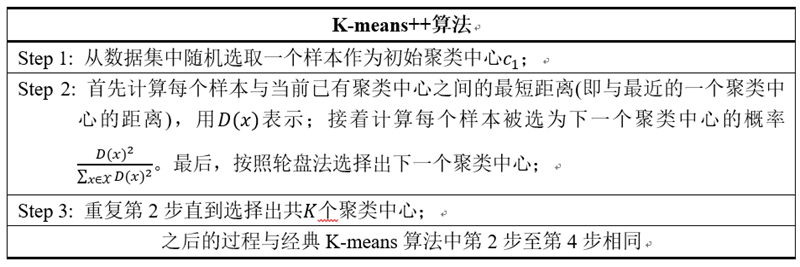
Solution: Kmeans++

Can we prevent arbitrarily bad local minima?
- Randomly choose first center.
- Pick new center with prob. proportional to (r-c)
  (Contribution of $x$ to total error) 以距离为概率选择下一个中心点
- Repeat until $k$ centers.

下面结合一个简单的例子说明K-means++是如何选取初始聚类中心的。数据集中共有8个样本，分布以及对应序号如下图所示：

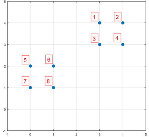
假设经过图2的步骤一后6号点被选择为第一个初始聚类中心，那在进行步骤二时每个样本的D(x)和被选择为第二个聚类中心的概率如下表所示：

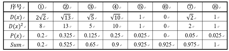
其中的P(x)就是每个样本被选为下一个聚类中心的概率。最后一行的Sum是概率P(x)的累加和，用于轮盘法选择出第二个聚类中心。方法是随机产生出一个0~1之间的随机数，判断它属于哪个区间，那么该区间对应的序号就是被选择出来的第二个聚类中心了。例如1号点的区间为[0,0.2)，2号点的区间为[0.2, 0.525)。
从上表可以直观的看到第二个初始聚类中心是1号，2号，3号，4号中的一个的概率为0.9。而这4个点正好是离第一个初始聚类中心6号点较远的四个点。这也验证了K-means的改进思想：即离当前已有聚类中心较远的点有更大的概率被选为下一个聚类中心。可以看到，该例的K值取2是比较合适的。
当K值大于2时，每个样本会有多个距离，需要取最小的那个距离作为D(x)。一开始只有一个中心，之后会有下一个，那么此时每个点都要遍历两个中心，则距离取最小值即可，物理意义就是希望下一个中心尽可能离这两个中心远一点
下面是选择中心点的代码

# coding: utf-8
import math
import random
from sklearn import datasets

def euler_distance(point1: list, point2: list) -> float:
    """
    计算两点之间的欧拉距离，支持多维
    """
    distance = 0.0
    for a, b in zip(point1, point2):
        distance += math.pow(a - b, 2)
    return math.sqrt(distance)

def get_closest_dist(point, centroids):
    min_dist = math.inf  # 初始设为无穷大
    for i, centroid in enumerate(centroids):
        dist = euler_distance(centroid, point)
        if dist < min_dist:
            min_dist = dist
    return min_dist

def kpp_centers(data_set: list, k: int) -> list:
    """
    从数据集中返回 k 个对象可作为质心
    """
    cluster_centers = []
    cluster_centers.append(random.choice(data_set))
    d = [0 for _ in range(len(data_set))]
    for _ in range(1, k):
        total = 0.0
        for i, point in enumerate(data_set):
            d[i] = get_closest_dist(point, cluster_centers) # 与最近一个聚类中心的距离
            total += d[i]
        total *= random.random()
        for i, di in enumerate(d): # 轮盘法选出下一个聚类中心；
            total -= di
            if total > 0:
                continue
            cluster_centers.append(data_set[i])
            break
    return cluster_centers

if __name__ == "__main__":
    iris = datasets.load_iris()
    print(kpp_centers(iris.data, 4))

5.3.2 spherical cluster

Will it always find the true patterns in the data?
- 不一定，他只能找到球状分布
- if the patterns are very clear?

Solution: GMM

A probabilistic variant of Kimeans:

E step: “soft assignment”of points to clusters （标记属于某个类的概率）
- estimate probability that a point is in a cluster
  - 先随机初始化一个概率分布，就可以计算每个点归类的概率
Mstep: update cluster parameters
- mean and variance info (covariance matrix)
- maximizes the likelihood of the points given the clusters

理论上足够多的高斯分布可以拟合任意数据点
详细见参考阅读GMM

5.3.3 How to choose the number of clusters?

Try different numbers of clusters in a validation set and look at performance.
We can plot the objective function values for k equals 1 to 6…
The abrupt change at k = 2, is highly suggestive of two clustersin the data. This technique for determining the number of clusters is known as “knee finding or “elbow finding.

6. Smoothing Out Cluster Assignments

聚类目标内部不连续

引入空间坐标的信息
K-means clustering based on intensity or color is essentially vector quantization（量化） of the image attributes
- 基于强度或颜色的K均值聚类本质上是矢量量化(量化）图像属性的分类
Clusters don’t have to be spatially coherent （空间相关性）

6.1 Spatial Coherence

Way to encode both similarity and proximity.
实际上就是在原本三维向量的基础上，多加两维空间信息

7. Mean-Shift Segmentation

An advanced and versatile technique for clustering-based segmentation

7.1 Algorithm 找到区域空间密度的极大值

随机初始化一个圆，然后找到点的重心，再以该重心为中心做圆，从而达到漂移的效果

在一个 n 维空间内，存在一个点 x，以该点为球心，以 h 为半径，生成一个球 $S_h$，计算球心到球内所有点生成的向量的均值，显然这个均值也是一个向量，这个向量就是 mean shift 向量
公式如下:

$M_{h}(x)=\frac{1}{k} \sum_{x_{i} \in S_{h}}\left(x_{i}-x\right)$

可以这么理解以上公式，我们定义了一个叫mean-shift的东西，它用于计算漂移距离

7.2 shift point

我给起个名字，叫偏移点；
注意，几乎没有资料专门提到这个概念，我为什么要讲呢？因为我们需要把 shift point 和 mean shift 区分开，这俩可不是一回事；
而在我们写算法时，需要的是 shift point，而不是 mean shift

$\hat{M}_n(X)=\frac{1}{k}(x_i),\text{shift point}$

7.3 基本思想

对于样本中的每一个点 $x$，做如下操作
以 x 为起点，计算他的 $\text{shift point } x’$，然后把该点 “移动” 到 x’.【注意不是真的移动点，而是把 x 标记成 x’】
以 $x’ $为新起点，计算他的 shift point
重复前两步，直至前后两次的 mean shift 向量满足条件，如距离很近【这一步才用到 mean shift，也就是前后两个 shift point 相减得到向量，再计算向量的模】
把 $x$ 标记为最终的 shift point，即为对应的类
遍历计算所有点

过程大致如下图：

从上图可以看到，mean shift 向量指向了更密集的区域，也就是说 mean shift 算法是在寻找最密集的区域，作为最后的类别
存在问题
- 在计算 mean shift 向量时，圆圈内所有点的贡献是一样的即1/k，而实际上离圆心越远可能贡献越小，
- 为此 mean shift 算法引入核函数来表达这种贡献，代替 1/k

7.4 引入核函数

此处以高斯核函数为例

$N(x)=\frac{1}{\sqrt{2 \pi} h} e^{-\frac{x^{2}}{2 h^{2}}}$

其中 h 代表核函数的带宽(bandwidth)【这个 h 和高斯分布里的标准差σ 类似，但它不是标准差，而是人工指定的，但是起到的作用和标准差一样】
h 越小，衰减为 0 的速度就越快，也就是说 mean shift 向量对应的球 Sh 越小，稍微远点就没有贡献了；
于是，引入核函数的 mean shift 向量变成如下样子，此时的 Sh 可以为整个数据集（原因为上句）

$M_{h}(x)=\frac{\sum_{i=1}^{n} G\left(\frac{x_{i}-x}{h_{i}}\right)\left(x_{i}-x\right)}{\sum_{i=1}^{n} G\left(\frac{x_{i}-x}{h_{i}}\right)}$

代码见：Mean shift 【1】- 基本原理 - 努力的孔子 - 博客园 (cnblogs.com)

证明：

7.4 如何聚类

Cluster: all data points in the attraction basin of amode
- 模式吸引区中的所有数据点
Attraction basin (吸引池): the region for which all trajectories（轨迹） lead to the same mode
- 对于指定一片区域，该区域中所有点最终会漂移到同一个点，这个区域被称为吸引区
- 遍历所有数据点，最后数据点最终漂移到哪一个中心，那么最后就是属于哪一个类

7.5 如何在数字图像上应用？

Find features (color, gradients, texture, etc)
Initialize windows at individual pixel locations 在各个像素位置初始化window
Perform mean shift for each window until convergence
Merge windows that end up near the same “peak” or mode 合并峰值点
- 可以理解为，虽然一开始生成了很多window，但是最终对于峰值接近的重心点，我们可以进行合并

7.6 speedups

遍历所有点，速度太慢

我们可以定义对于圆内r/c部分的点和中心点都会最终漂移到同一个点，那么这部分点就不用再遍历

一开始初始化多个圆，然后依次进行漂移，从而实现聚类

7.7 Summary Mean-Shift

Pros
- General, application-independent tool
- Model-free, does not assume any prior shape (spherical, elliptical, etc.)on data clusters
- Just a single parameter (window size h)
  - h has a physical meaning (unlike k-means)·
- Finds variable number of modes
- Robust to outliers
Cons
- Output depends on window size
- Computationally (relatively) expensive

8. Graph-based segmentation

8.1 Efficient graph-based segmentation

Runs in time nearly linear in the number of edges
- 时间复杂度和边数相关
Easy to control coarseness（粗糙度） of segmentations
Results can be unstable

8.2 Segmentation by graph cuts

断掉某些边，把没连通的集合分为两类

A graph cut is a set of edges whose removal disconnects the graph
- 图割是一个从原图断掉联系的边集，去掉该边集，会使得原图不在连通即不相连
Cost of a cut: sum of weights of cut edges
- 即图割中所有边的权值和

断掉相似度最小的边

8.3 Measuring affinity（亲和力）（定义相似度）

One possibility:
- 特征上的距离差异，与相似度成反比

$a f f(x, y)=\exp (-\frac{\|x-y\|^{2}}{2 \sigma_{d}^{2}})$

8.4 Cuts in a graph: Min cut 最小割

Link Cut: set of links whose removal makes a graph disconnected
cost of a cut:
$\operatorname{cut}(A, B)=\sum_{p \in A, q \in B} w_{p, q}$
Find minimum cut：
gives you a segmentation
fast algorithms exist for doing this
- 断掉的权重值之和最小

8.5 Problem

Minimum cut tends to cut off very small, isolated components
- 容易造成孤立点分割，因为这些点可能和其他点的相似度都很低，所以自然就被切割走了·

8.6 Cuts in a graph: Normalized cut

Normalized Cut

fix bias of Min Cut by normalizing for size of segments: $N \operatorname{cut}(A, B)=\frac{\operatorname{cut}(A, B)}{\operatorname{assoc}(A, V)}+\frac{\operatorname{cut}(A, B)}{\operatorname{assoc}(B, V)}$
$\operatorname{assoc}(\mathrm{A}, \mathrm{V})=$ sum of weights of all edges that touch $\mathrm{A}$
- 即除以割开后，分别处以两个图的权重之和，再相加
- 这样可以使得，分割后的连个cluster的权重之和尽可能均衡
Ncut value small when we get two clusters with many edges with high weights, and few edges of low weight between them
- 尽可能使得同一类多边
Approximate solution for minimizing the Ncut value : generalized eigenvalue problem.
- 求解方法：广义特征值

8.7 Normalized cuts: Pro and con

Pro

Generic framework, can be used with many different features and affinity formulations

Con

High storage requirement and time complexity:
- involves solving a generalized eigenvalue problem of size $n \times n$, where n is the number of pixels

9. Feature Space

Depending on what we choose as the feature space, we can group pixels in different ways.
Grouping pixels based on color similarity

color, brightness, position alone are not enough to distinguish all regions…

9.1 Recall: texture representation example

分别计算一个小窗口里水平方向梯度的均值以及垂直方向梯度的均值，作为这个小窗口的特征，再进行聚类

9.2 Segmentation with texture features

Find “textons” （文本） by clustering vectors of filter bank outputs.
- 查找“内容” 通过对滤波器组输出向量进行聚类。
Describe texture in a window based on texton histogram
- 对于每个小窗口，我们可以得到多个filter在该小窗口的多个值，我们可以以filtter为横坐标建立直方图

9.3 lmage segmentation example

利用多特征融合，实现通过不同特征分割的手段，融合出较好的图像分割结果

9.4 Segments as primitives for recognition

一辆车可能方位形状不一样，且经常有遮挡，但我们也要完成这个任务

10. Summary

Segmentation to find object boundaries or mid-level regions,tokens.
Bottom-up segmentation via clustering
General choices — features, affinity functions, and clustering algorith ms
Grouping also useful for quantization, can create new featuresummaries
Texton histograms for texture within local region·
Example clustering methods
- K-means
- Mean shift
- Graph cut, normalized cuts